Soft crawling robot

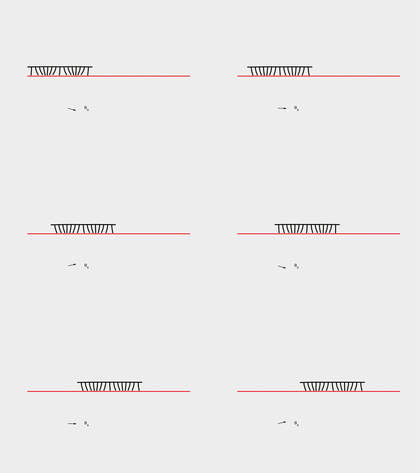
In this subsection, we present the frictional contact interaction of a soft crawling robot with multiple legs as it moves across a surface under external magnetic actuation. Using the DDG simulation framework, we analyze how the legs interact with the ground, generating propulsion through controlled frictional forces. The interplay between magnetic excitation, elastic deformation, and contact dynamics determines the robot’s locomotion efficiency and stability. By capturing the complex coupling between actuation and ground interaction, this model provides valuable insights into the design of magnetically controlled soft robots for applications in biomedical engineering, inspection, and search-and-rescue operations.

Simulation Initialization

To initialize the simulation, the following inputs are used:

1. Geometry and connection:
   • (i) Nodal positions: the position of the nodes \(\mathbf{q}(t=0)\), with a total of \(N = 169\). The robot’s body trunk is a magnetized beam with a length of \(L = 0.08\mathrm{~m}\), and it has 15 limbs, each also a magnetized beam with a length of \(L_0 = 0.0134\mathrm{~m}\).
   • (ii) Stretching elements: the connections between the nodes, with a total of \(N_s = 168\).
   • (iii) Bending elements: the connections between the edges, with a total of \(N_b = 182\).
2. Physical parameters:
   • (i) Young’s modulus, \(E = 1.0\mathrm{~MPa}\).
   • (ii) Material density, \(\rho = 1000\) \(\mathrm{kg/m^3}\).
   • (iii) Cross-sectional radius, \(r_0 = 0.001\mathrm{~m}\).
   • (iv) Damping viscosity, \(\mu = 0.1\).
   • (v) Gravity, \(\mathbf{g} = [0.0, -10]^{T}\) \(\mathrm{m/s^2}\).
   • (vi) The leg magnetization is \(B_r^x = 1000 \cos(4 \pi s)\), \(B_r^y = 1000 \sin(4 \pi s)\), where \(s \in [0,1]\) is the arc length parameter of the robotic body.
   • (vii) Contact parameters, including \(\hat{d} = 1 \times 10^{-3}\mathrm{~m}\), \(K_c = 1.0\mathrm{~kPa}\), \(\mu = 0.3\), and \(\epsilon_v = 1 \times 10^{-6}\mathrm{~m/s}\).
3. Numerical parameters:
   • (i) Total simulation time, \(T = 2.0\mathrm{~s}\).
   • (ii) Time step size, \(\mathrm{dt} = 0.001\mathrm{~s}\).
   • (iii) Numerical tolerance, \(\mathrm{tol} = 1 \times 10^{-4}\).
   • (iv) Maximum iterations, \(N_{\mathrm{iter}} = 10\).
4. Boundary conditions:
   • No nodes are constrained in this case, thus the constrained array is \(\mathcal{FIX} = \emptyset\).
5. Initial conditions:
   • (i) Initial position is input from the nodal positions.
   • (ii) Initial velocity is set to zeros for all nodes.
6. Loading steps:
   • A magnetic field with \(B_x = A \cos(\omega t)\) and \(B_y = A \sin(\omega t)\) (with \(A = 1.0\mathrm{~T}\) and \(\omega = 10\pi\mathrm{~rad/s}\)) is applied to the entire robotic system.

Dynamic Rendering