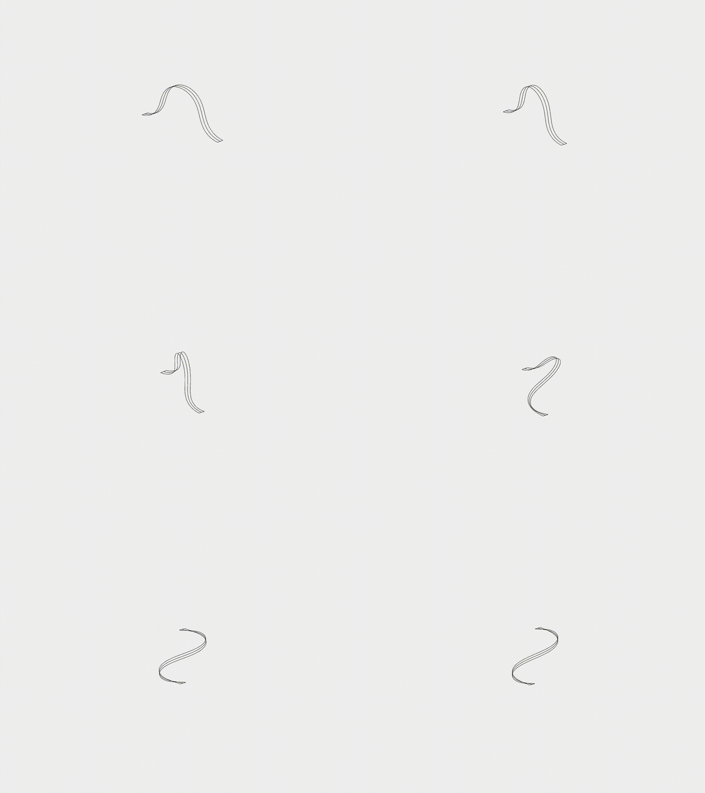
Bifurcation of pre-buckled ribbon

The shear deformation behavior of a pre-buckled ribbon exhibits bifurcation characteristics. The continuation method is commonly used to trace the deformation path, particularly for identifying static bifurcation critical points, while dynamic bifurcation behavior has been explored using the Discrete Elastic Rod (DER) model in prior studies. In this case study, we investigate the shear deformation of a pre-buckled ribbon under clamped-clamped boundary conditions, incorporating specific loading conditions into the simulation. The deformation pathway is tracked, identifying critical instability and stability points. This case demonstrates the capability of the DDG model to capture complex bifurcation characteristics in slender structures subjected to shear deformation.

Simulation Initialization

To initialize the simulation, the following inputs are used:

1. Geometry and connection:
   • (i) Nodal positions: the position of the nodes, \(\mathbf{q}(t=0)\), with a total of \(N=50\). The rod is initialized as a flat ribbon with a length \(L=1.0\mathrm{~m}\).
   • (ii) Stretching elements: connection of every two consecutive nodes, for a total of \(N_{s}=49\).
   • (iii) Bending elements: connection of every two consecutive edges, for a total of \(N_{b}=48\).
2. Physical parameters:
   • (i) Young’s modulus, \(E=100.0\mathrm{~MPa}\).
   • (ii) Poisson’s ratio, \(\nu=0.5\).
   • (iii) Material density, \(\rho=1000\mathrm{~kg/m^3}\).
   • (iv) Ribbon width, \(w=0.2\mathrm{~m}\); Ribbon thickness, \(h=0.01\mathrm{~m}\). Thus, \(EI_{2} = Ewh^3/12\), \(EI_{1} = 400EI_{2}\), and \(GJ = Gwh^3/3\).
   • (v) Damping viscosity, \(\mu = 0.1\).
   • (vi) The overall simulation is static, i.e., \(\mathrm{ifStatic} = 1\).
3. Numerical parameters:
   • (i) Total simulation time, \(T=40.0\mathrm{~s}\).
   • (ii) Time step size, \(\mathrm{dt} = 0.01\mathrm{~s}\).
   • (iii) Numerical tolerance, \(\mathrm{tol} = 1 \times 10^{-4}\).
   • (iv) Maximum iterations, \(N_{\mathrm{iter}} = 10\).
4. Boundary conditions:
   • The first two nodes and the last two nodes, \(\{\mathbf{x}_{1},\mathbf{x}_{2},\mathbf{x}_{49},\mathbf{x}_{50} \}\), as well as the first twisting angle and the last twisting angle, \(\{\theta_{1}, \theta_{49}\}\), are fixed to achieve clamped-clamped boundary conditions. Thus, the constrained array is: \(\mathcal{FIX} = [1,2,3,4,5,6,147,148,149,150,151,199]^{T}\).
5. Initial conditions:
   • (i) Initial position is input from the nodal positions.
   • (ii) Initial velocity is set to zeros.
6. Loading steps:
   • (i) Compression step: For \(t \leq 3.0\mathrm{~s}\), a displacement is applied to both ends along the \(X\)-axis with speed \(v_{x} = 0.1\mathrm{~m/s}\), until the compressive distance reaches \(\Delta X \geq 0.4\mathrm{~m}\). To induce the bifurcation direction, the gravity vector is set as: \(\mathbf{g}=[0.0,0.0,10.0]^T\mathrm{~m/s^2}\).
   • (ii) Change perturbation: For \(3.0\mathrm{~s} \leq t \leq 5.0\mathrm{~s}\), the gravity force is switched to: \(\mathbf{g}=[0.1,0.1,0.0]^T\mathrm{~m/s^2}\) to change the perturbation direction.
   • (iii) Shear step: For \(t \geq 5.0\mathrm{~s}\), a displacement is applied to both ends along the \(Y\)-axis with speed \(v_{y} = 0.01\mathrm{~m/s}\), until the shear distance reaches \(\Delta Y \geq 0.6\mathrm{~m}\).

Dynamic Rendering