Rod and ribbon: 3D curve
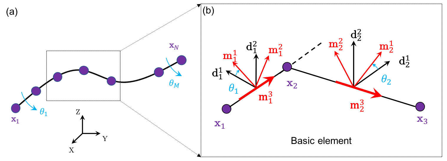
Here, we formulate the mechanics of 3D slender structures, such as rods or ribbons, whose motion can be simplified to that of a central line, represented as a 3D curve. As shown in the figure below, to capture the configuration of the curve, we need \(N\) nodes and \(M\) edges. Each node is denoted as \(\mathbf{x}_{i} \equiv [x_{i}, y_{i}, z_{i}]^{T} \in \mathcal{R}^{3 \times 1}\). To define an edge, two frames are required: for the \(j\)-th edge, we introduce an adaptive reference frame, \(\{ \mathbf{d}_{j}^{1}, \mathbf{d}_{j}^{2}, \mathbf{d}_{j}^{3}\}\), and a local material frame, \(\{ \mathbf{m}_{j}^{1}, \mathbf{m}_{j}^{2}, \mathbf{m}_{j}^{3}\}\). These frames share a common tangent direction, and the rotational angle between the two frames along the tangent direction is defined as \(\theta_{j}\), i.e.
\[\mathbf{m}_{j}^{1} = \mathbf{d}_{j}^{1} \cos(\theta_{j}) + \mathbf{d}_{j}^{2} \sin(\theta_{j}), \; \mathbf{m}_{j}^{2} = \mathbf{d}_{j}^{2} \cos(\theta_{j}) -\mathbf{d}_{j}^{1} \sin(\theta_{j}), \; \mathbf{m}_{j}^{3} \equiv \mathbf{d}_{j}^{3}.\]The total DOF vector is defined as
\[\mathbf{q} = [ \mathbf{x}_1; \mathbf{x}_2; \ldots; {\mathbf{x}_{N}}; \theta_{1}; \theta_{2}; \ldots; \theta_{M} ] \in \mathcal{R}^{ (3N+M) \times 1}.\]Three types of elements are used to capture the mechanics of a discrete slender structure in 3D space: (i) stretching element, (ii) bending element, and (iii) twisting element. Consistent with the previous section, the number of stretching elements is denoted as \(N_{s}\), while the number of bending and twisting elements are the same and denoted as \(N_{b}\). Similar to the previous planar beam case, if only the stretching element is considered, the 3D rod structures would reduce to the 3D cable structures.
Stretching element
The stretching element is comprised of two connected nodes, defined as
\[\mathcal{S}: \{\mathbf{x}_{1}, \mathbf{x}_{2}, \theta_{1} \}.\]As the formulation of stretching strain is independent of the twisting angle, \(\theta_{1}\), the local DOF vector depends only on the nodes and is defined as
\[\mathbf{q}^{s} \equiv [\mathbf{x}_{1}; \mathbf{x}_{2} ] \in \mathcal{R}^{6 \times 1}.\]The edge length is the \(\mathcal{L}_{2}\) norm of the edge vector, defined as
\[l = || \mathbf{x}_{2} -\mathbf{x}_{1} ||.\]The stretching strain is based on the uniaxial elongation of the edge, defined as
\[{\varepsilon} = \frac { l } { \bar{l} } - 1.\]Hereafter, we use a bar on top to indicate the evaluation of the undeformed configuration, e.g., \(\bar{l}\) is the edge length before deformation. Using the linear elastic model, the total stretching energy is expressed as a quadratic function of the strain following the linear elastic constitutive law
\[E^s = \frac{1}{2} EA (\varepsilon)^2 \bar{l},\]where \(EA\) is the local stretching stiffness. The local stretching force vector, \(\mathbf{F}^{s}_{\mathrm{local}} \in \mathcal{R}^{6 \times 1}\), as well as the local stretching Hessian matrix, \(\mathbb{K}^{s}_{\mathrm{local}} \in \mathcal{R}^{6 \times 6}\), can be derived through a variational approach as
\[\mathbf{F}^{s}_{\mathrm{local}} = -\frac{\partial E^{s}} {\partial \mathbf{q}^{s}}, \; \mathrm{and} \; \mathbb{K}^{s}_{\mathrm{local}} = \frac {\partial^2 E^{s}} {\partial \mathbf{q}^{s} \partial \mathbf{q}^{s}}.\]The detailed formulation can be found in the MATLAB code. Finally, the global stretching force vector, \(\mathbf{F}^{s}\), and the associated Hessian matrix, \(\mathbb{K}^{s}\), can be assembled by iterating over all stretching elements.
Bending element
Similarly, we extend the bending element to a 3D discrete slender structure as
\[\mathcal{B}: \{ \mathcal{S}_{1}, \mathcal{S}_{2}\}, \; \mathrm{with} \; \mathcal{S}_{1} : \{ \mathbf{x}_{1}, \mathbf{x}_{2}, \theta_{1} \} \; \mathrm{and} \; \mathcal{S}_{2} : \{ \mathbf{x}_{2}, \mathbf{x}_{3}, \theta_{2} \}.\]Here, we define \(\mathbf{x}_{2}\) as the joint node, and \(\mathbf{x}_{1}\) and \(\mathbf{x}_{3}\) are the two adjacent nodes. Thus, the local DOF vector is defined as
\[\mathbf{q}_{b} \equiv [\mathbf{x}_{1}; \mathbf{x}_{2}; \mathbf{x}_{3}; \theta_{1};\theta_{2} ] \in \mathcal{R}^{11 \times 1}.\]The two edge vectors are
\[\mathbf{e}_{1} = \mathbf{x}_{2} -\mathbf{x}_{1}, \; \mathbf{e}_{2} = \mathbf{x}_{3} -\mathbf{x}_{2}.\]The Voronoi length of the bending element is the average of the two edges, defined as
\[l = \frac{1} {2}( || \mathbf{e}_{1} || + || \mathbf{e}_{2} || ).\]The curvature bi-normal, which measures the misalignment between two consecutive edges at the center node, is given by
\[\kappa \mathbf{b}=\frac{2\;\mathbf{e}_1\times \mathbf{e}_2}{\mathbf{e}_1\cdot \mathbf{e}_2+\left\| \mathbf{e}_1 \right\| \left\| \mathbf{e}_2 \right\|}.\]The material curvatures are given by the inner products between the curvature bi-normal and the material frame as
\[\kappa_{1} = \frac {\kappa \mathbf{b}} {2} \cdot \frac {\left( \mathbf m_1^{2} + \mathbf m_2^{2} \right)} { l}, \; \kappa_{2} = - \frac {\kappa \mathbf{b}} {2} \cdot \frac{\left( \mathbf m_1^{1} + \mathbf m_2^{1}\right) } { l}.\]For the linear elastic constitutive model, the discrete bending energy is a quadratic function of the curvature as
\[E^{b} = \frac{1}{2} EI_{1} {(\kappa_{1} - \bar{\kappa}_{1})^2 } \bar{l} + \frac{1}{2} EI_{2} {(\kappa_{2} - \bar{\kappa}_{2})^2 } \bar{l},\]where \(EI_{1}\) and \(EI_{2}\) are the local bending stiffness along the two bending axes of the section, respectively. The local bending force vector, \(\mathbf{F}^{b}_{\mathrm{local}} \in \mathcal{R}^{11 \times 1}\), as well as the local bending Hessian matrix, \(\mathbb{K}^{b}_{\mathrm{local}} \in \mathcal{R}^{11 \times 11}\), can be derived through a variational approach as
\[\mathbf{F}^{b}_{\mathrm{local}} = -\frac{\partial E^{b}} {\partial \mathbf{q}^{b}}, \; \mathrm{and} \; \mathbb{K}^{b}_{\mathrm{local}} = \frac {\partial^2 E^{b}} {\partial \mathbf{q}^{b} \partial \mathbf{q}^{b}}.\]The detailed formulation can be found in the MATLAB code. Finally, the global bending force vector, \(\mathbf{F}^{b}\), and the associated Hessian, \(\mathbb{K}^{b}\), can be assembled by iterating over all bending elements.
Twisting energy
Here, we define the twist for a 3D slender structure. Similar to the bending element, the twisting element is defined as
\[\mathcal{T} \equiv \mathcal{B}: \{ \mathcal{S}_{1}, \mathcal{S}_{2}\}, \; \mathrm{with} \; \mathcal{S}_{1} : \{ \mathbf{x}_{1}, \mathbf{x}_{2}, \theta_{1} \} \; \mathrm{and} \; \mathcal{S}_{2} : \{ \mathbf{x}_{2}, \mathbf{x}_{3}, \theta_{2} \}.\]The local DOF vector is defined as
\[\mathbf{q}^{t} \equiv [\mathbf{x}_{1}; \mathbf{x}_{2}; \mathbf{x}_{3}; \theta_{1}; \theta_{2} ] \in \mathcal{R}^{11 \times 1}.\]The twisting curvature is the sum of the twist of the reference frame, \(\tau_{r}\), and the twist of the material frame, \(\tau_{m}\),
\[\tau = \tau_{\mathrm{r}} + \tau_{\mathrm{m}},\]where
\[\tau_{\mathrm{m}} = \frac {\theta_{2} - \theta_{1}} {l},\]and the formulation of the reference twist, \(\tau_{r}\), can be found in our paper. Finally, for a linear elastic constitutive, the discrete twisting energy is given by
\[E_{t} = \frac{1}{2} GJ {(\tau - \bar{\tau})^2 } \bar{l},\]where \(GJ\) is the local twisting stiffness. The local twisting force vector, \(\mathbf{F}^{t}_{\mathrm{local}} \in \mathcal{R}^{11 \times 1}\), as well as the local bending Hessian matrix, \(\mathbb{K}^{t}_{\mathrm{local}} \in \mathcal{R}^{11 \times 11}\), can be derived through a variational approach as
\[\mathbf{F}^{t}_{\mathrm{local}} = -\frac{\partial E^{t}} {\partial \mathbf{q}^{t}}, \; \mathrm{and} \; \mathbb{K}^{t}_{\mathrm{local}} = \frac {\partial^2 E^{t}} {\partial \mathbf{q}^{t} \partial \mathbf{q}^{t} }.\]The detailed formulation can be found in the MATLAB code. Finally, the global twisting force vector, \(\mathbf{F}^{t}\), and the associated Hessian, \(\mathbb{K}^{t}\), can be assembled by iterating over all twisting elements.