Beam: planar curve
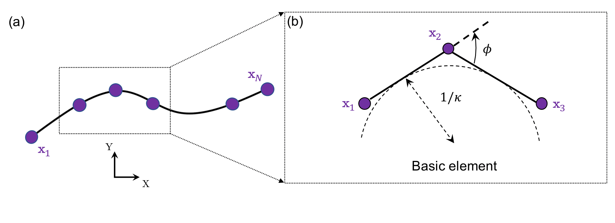
As shown in the figure below, the configuration of a planar beam is described by \(N\) nodes, where each node is defined as \(\mathbf{x}_{i} \equiv [x_{i}, y_{i}]^{T} \in \mathcal{R}^{2 \times 1}\). Therefore, the DOF vector can be expressed as:
\[\mathbf{q} = \left[ \mathbf{x}_1; \mathbf{x}_2; \ldots; {\mathbf{x}_{N}} \right] \in \mathcal{R}^{2N \times 1}.\]Two types of elements are used to capture the total elastic energies of a discrete planar beam: (i) stretching element and (ii) bending element, with \(N_{s}\) and \(N_{b}\) representing the number of each, respectively. Note that if only the stretching element is considered, the bending-dominated beam structures would reduce to the stretching-dominated cable structures.
Stretching element
The stretching element is comprised of two connected nodes, defined as:
\[\mathcal{S}: \{\mathbf{x}_{1}, \mathbf{x}_{2} \}.\]Hereafter, we omit the subscript \(i\) for simplicity. The local DOF vector of the stretching element is defined as:
\[\mathbf{q}^{s} \equiv [\mathbf{x}_{1}; \mathbf{x}_{2} ] \in \mathcal{R}^{4 \times 1}.\]The edge length is the \(\mathcal{L}_{2}\) norm of the edge vector, defined as:
\[l = || \mathbf{x}_{2} - \mathbf{x}_{1} ||.\]The stretching strain is based on the uniaxial elongation of the edge, defined as:
\[{\varepsilon} = \frac{l}{\bar{l}} - 1.\]Using the linear elastic model, the total stretching energy is expressed as a quadratic function of the strain:
\[E^s = \frac{1}{2} EA (\varepsilon)^2 \bar{l},\]where \(EA\) is the local stretching stiffness. The local stretching force vector and Hessian matrix can be derived through a variational approach:
\[\mathbf{F}^{s}_{\mathrm{local}} = -\frac{\partial E^{s}}{\partial \mathbf{q}^{s}}, \quad \mathbb{K}^{s}_{\mathrm{local}} = \frac{\partial^2 E^{s}}{\partial \mathbf{q}^{s} \partial \mathbf{q}^{s}}.\]The detailed formulation can be found in the MATLAB code. Finally, the global stretching force vector, \(\mathbf{F}^{s}\), and the associated Hessian matrix, \(\mathbb{K}^{s}\), can be assembled by iterating over all stretching elements.
Bending element
Similarly, the bending element consists of two consecutive edges sharing a common node:
\[\mathcal{B}: \{ \mathcal{S}_{1}, \mathcal{S}_{2}\}, \quad \mathcal{S}_{1} : \{ \mathbf{x}_{1}, \mathbf{x}_{2} \}, \quad \mathcal{S}_{2} : \{ \mathbf{x}_{2}, \mathbf{x}_{3} \}.\]The local DOF vector is:
\[\mathbf{q}^{b} \equiv [\mathbf{x}_{1}; \mathbf{x}_{2}; \mathbf{x}_{3} ] \in \mathcal{R}^{6 \times 1}.\]The two edge vectors are:
\[\mathbf{e}_{1} = \mathbf{x}_{2} - \mathbf{x}_{1}, \quad \mathbf{e}_{2} = \mathbf{x}_{3} - \mathbf{x}_{2}.\]The Voronoi length of the bending element is:
\[l = \frac{1}{2} \left( || \mathbf{e}_{1} || + || \mathbf{e}_{2} || \right).\]The bending curvature is associated with the turning angle between the two connecting edges:
\[{\kappa} = \frac{2 \tan \left( \frac{\phi}{2} \right)}{l}.\]The discrete bending energy is given by:
\[E^{b} = \frac{1}{2} EI (\kappa - \bar{\kappa})^2 \bar{l},\]where \(EI\) represents the local bending stiffness. The local bending force vector and Hessian matrix are derived using a variational approach:
\[\mathbf{F}^{b}_{\mathrm{local}} = -\frac{\partial E^{b}}{\partial \mathbf{q}^{b}}, \quad \mathbb{K}^{b}_{\mathrm{local}} = \frac{\partial^2 E^{b}}{\partial \mathbf{q}^{b} \partial \mathbf{q}^{b}}.\]The detailed formulation can be found in the MATLAB code. Finally, the global bending force vector, \(\mathbf{F}^{b}\), and the associated Hessian, \(\mathbb{K}^{b}\), can be assembled by iterating over all c elements.