Axisymmetric shell: rotational surface
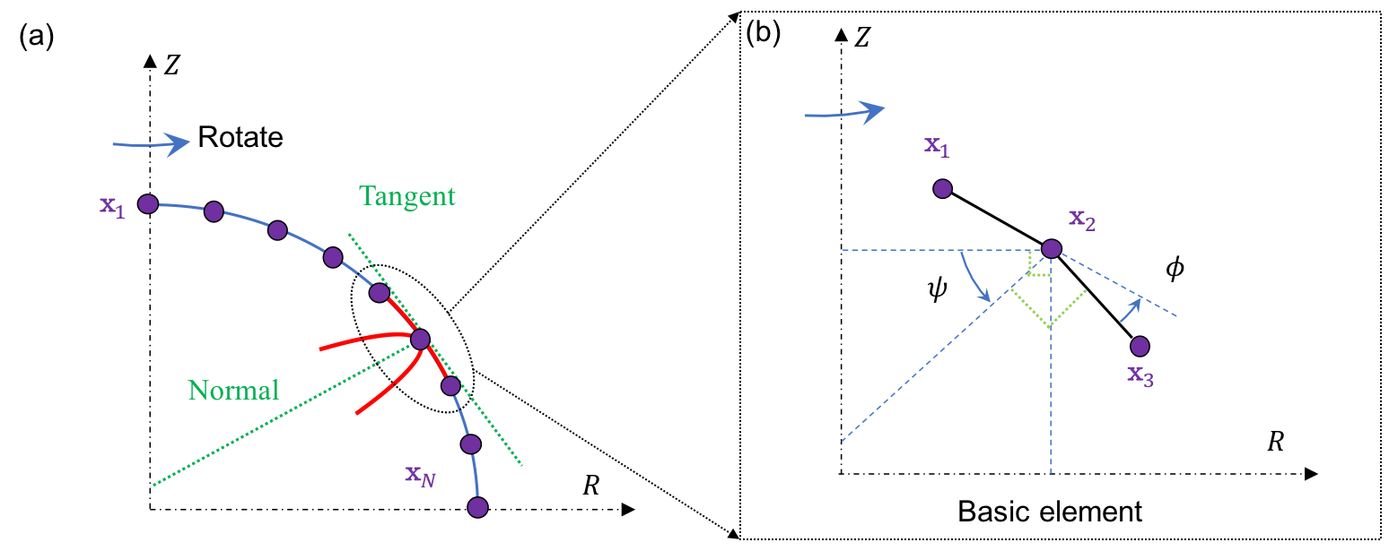
Here, we discuss how a simple 2D curve can represent the mechanics of an axisymmetric structure. As shown in the figure below, the configuration of a rotational symmetric curve is presented by \(N\) nodes, where each node is defined as \(\mathbf{x}_{i} \equiv [r_{i}, z_{i}]^{T} \in \mathcal{R}^{2 \times 1}\). Consequently, the total DOF vector is given by
\[\mathbf{q} = [ \mathbf{x}_1; \mathbf{x}_2; \ldots; {\mathbf{x}_{N}} ] \in \mathcal{R}^{2N \times 1}.\]Two types of elements are used to capture the mechanics of a rotational surface: (i) stretching element, and (ii) bending element. The number of stretching elements is denoted as \(N_{s}\), while the number of bending elements is denoted as \(N_{b}\). If only the stretching element is considered, the bending-dominated plate/shell structures would be reduced to the stretching-dominated membrane structures.
Stretching element
The stretching element is comprised of two connected nodes, defined as
\[\mathcal{S}: \{\mathbf{x}_{1}, \mathbf{x}_{2} \}.\]The local DOF vector is defined as
\[\mathbf{q}^{s} \equiv [\mathbf{x}_{1}; \mathbf{x}_{2} ] \in \mathcal{R}^{4 \times 1}.\]The edge length is the \(\mathcal{L}_{2}\) norm of the edge vector, defined as
\[l = || \mathbf{x}_{2} -\mathbf{x}_{1} ||.\]The average radius is
\[r =\frac{1}{2} (r_{1} + r_{2}).\]Thus, the total area of this stretching element is
\[s = 2 \pi r l.\]The element elongation along the meridional direction is straightforward, following the same formulation as the planar beam, given by
\[{\varepsilon}_{1} = \frac { l} { \bar{l} } - 1.\]Hereafter, we use a bar on top to indicate the evaluation of the undeformed configuration, e.g., \(\bar{l}\) is the edge length before deformation. The stretching along the circumferential direction is related to the radial expansion of the circle
\[{\varepsilon}_{2} = \frac { r } { \bar{r} } - 1,\]Due to the axisymmetric assumption, the shear coupling between the meridional direction and the circumferential direction is zero, i.e.,
\[{\varepsilon}_{12} ={\varepsilon}_{21} = 0.\]Using the linear elastic model, the total stretching energy follows a quadratic function of the strain,
\[E^s = \frac{1} {2} \frac {Eh} {1-\nu^2} \left( \varepsilon_{1}^2 + 2 \nu \varepsilon_{1} \varepsilon_{2} + \varepsilon_{2}^2 \right) \bar{s},\]where \(E\) is the young’s modulus, \(\nu\) is the Poisson ratio, and \(h\) is the shell thickness. The local stretching force vector, \(\mathbf{F}^{s}_{\mathrm{local}} \in \mathcal{R}^{4 \times 1}\), as well as the local stretching Hessian matrix, \(\mathbb{K}^{s}_{\mathrm{local}} \in \mathcal{R}^{4 \times 4}\), can be derived through a variational approach as
\[\mathbf{F}^{s}_{\mathrm{local}} = -\frac{\partial E^{s}} {\partial \mathbf{q}^{s}}, \; \mathrm{and} \; \mathbb{K}^{s}_{\mathrm{local}} = \frac {\partial^2 E^{s}} {\partial \mathbf{q}^{s} \partial \mathbf{q}^{s}}.\]The detailed formulation can be found in the MATLAB code. Finally, the global stretching force vector, \(\mathbf{F}^{s}\), and the associated Hessian matrix, \(\mathbb{K}^{s}\), can be assembled by iterating over all stretching elements.
Bending element
The bending element is comprised of two consecutive edges sharing a common node, defined as
\[\mathcal{B}: \{ \mathcal{S}_{1}, \mathcal{S}_{2}\}, \; \mathrm{with} \; \mathcal{S}_{1} : \{ \mathbf{x}_{1}, \mathbf{x}_{2} \} \; \mathrm{and} \; \mathcal{S}_{2} : \{ \mathbf{x}_{2}, \mathbf{x}_{3} \}.\]Here, we define \(\mathbf{x}_{2}\) as the joint node, and \(\mathbf{x}_{1}\) and \(\mathbf{x}_{3}\) are the two adjacent nodes. Thus, the local DOF vector is defined as
\[\mathbf{q}^{b} \equiv [\mathbf{x}_{1}; \mathbf{x}_{2}; \mathbf{x}_{3} ] \in \mathcal{R}^{6 \times 1}.\]The two edge vectors are
\[\begin{aligned} \mathbf{e}_{1} &= \mathbf{x}_{2} -\mathbf{x}_{1},\\ \mathbf{e}_{2} &= \mathbf{x}_{3} -\mathbf{x}_{2}. \end{aligned}\]The Voronoi length of the bending element is the average of the lengths of the two edges, defined as
\[l = \frac{1} {2}( || \mathbf{e}_{1} || + || \mathbf{e}_{2} || ).\]The local radius of the bending element is,
\[r = \frac{1} {3} (r_{1} + r_{2} + r_{3}).\]Thus, the total area is
\[s = 2 \pi r l.\]The meridional curvature is associated with the turning angle between the two connected edges as
\[\kappa_{1} = \frac { 2 \tan ( {\phi / {2} )}} { l },\]where \(\phi\) is the turning angle between the three consecutive nodes. The curvature along the circumferential direction is determined by the change in the surface’s normal direction, as
\[\kappa_{2} = \frac { \cos (\psi) } { r },\]where \(\psi\) is the orientation angle, determined by the surface normal vector relative to the \(R\) axis. Similarly, the bending coupling between the meridional direction and the circumferential direction is also zero, i.e.,
\[\kappa_{12} = \kappa_{21} = 0.\]The total bending energy is
\[E^b = \frac{1}{2} \frac {Eh^3} {12(1-\nu^2)} \left[ (\kappa_{1} - \bar{\kappa}_{1})^2 + 2 \nu (\kappa_{1} - \bar{\kappa}_{1}) (\kappa_{2} - \bar{\kappa}_{2}) + (\kappa_{2} - \bar{\kappa}_{2})^2 \right] \bar{s} .\]The local bending force vector, \(\mathbf{F}^{b}_{\mathrm{local}} \in \mathcal{R}^{6 \times 1}\), as well as the local bending Hessian matrix, \(\mathbb{K}^{s}_{\mathrm{local}} \in \mathcal{R}^{6 \times 6}\), can be derived through a variational approach as
\[\mathbf{F}^{b}_{\mathrm{local}} = -\frac{\partial E^{b}} {\partial \mathbf{q}^{b}}, \; \mathrm{and} \; \mathbb{K}^{b}_{\mathrm{local}} = \frac {\partial^2 E^{b}} {\partial \mathbf{q}^{b} \partial \mathbf{q}^{b}}.\]The detailed formulation can be found in the MATLAB code. Finally, the global bending force vector, \(\mathbf{F}^{b}\), and the associated Hessian, \(\mathbb{K}^{b}\), can be assembled by iterating over all stretching elements.