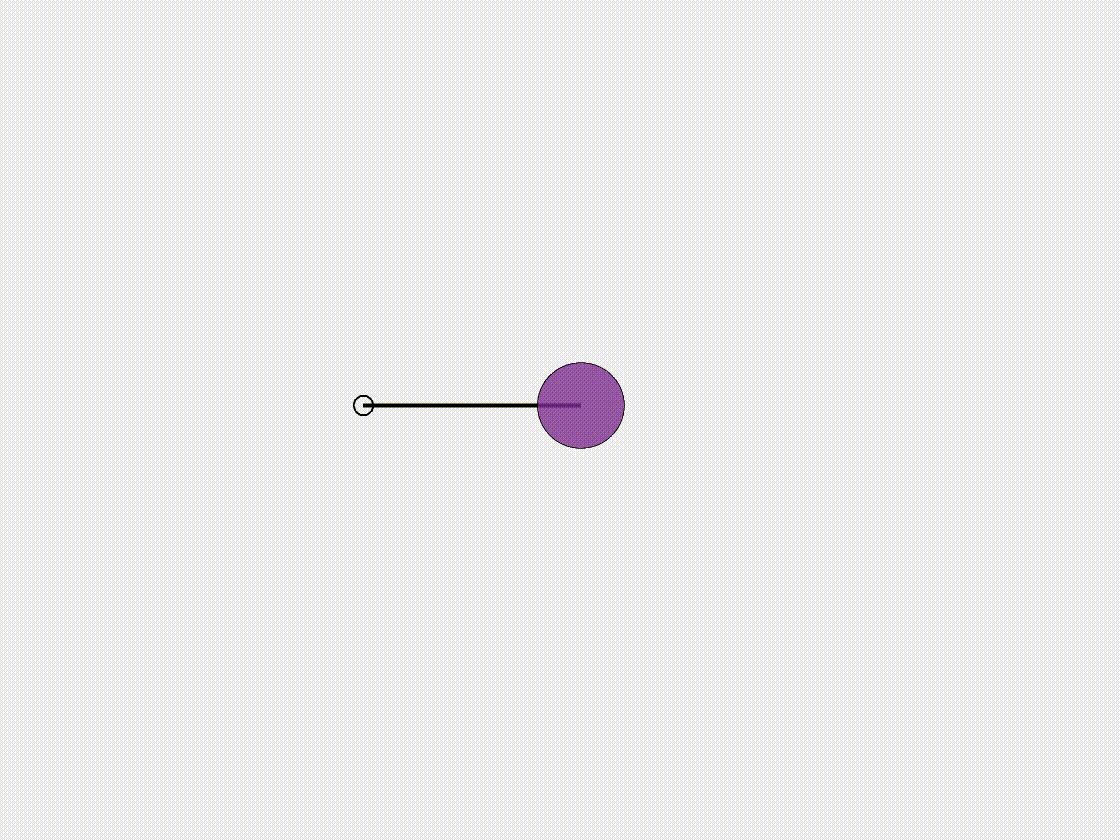
Single DOF mass-spring-damper system

We begin with the simplest case, a single-degree-of-freedom (S-DOF) mass-spring-damper system.

Simulation Initialization

To initialize the simulation, the following inputs are used:

1. Geometry and connection:
   • The spring length is \(l_0=1.0\mathrm{~m}\). Since there is only a single node, we only need to input its own initial position at \(x(t=0)=1.0\mathrm{~m}\), which is set to the spring’s equilibrium position \(x=l_0\) in this case.
2. Physical parameters:
   • (i) Mass \(m = 1.0\mathrm{~kg}\).
   • (ii) Damping viscosity \(c = 0.1\).
   • (iii) Spring stiffness \(k = 10.0\mathrm{~N/m}\).
3. Numerical parameters:
   • (i) Total simulation time \(T=10.0\mathrm{~s}\).
   • (ii) Time step size \(\mathrm{dt}=0.01\mathrm{~s}\).
   • (iii) Numerical force tolerance \(\mathrm{tol}=1\times 10^{-6}\).
4. Boundary conditions:
   • No boundary condition is applied for this simple S-DOF system.
5. Initial conditions:
   • (i) Initial position \(x(t=0) = 1.0 \mathrm{~m}\).
   • (ii) Initial velocity \(\dot{x}(t=0) = 0.0 \mathrm{~m/s}\).
6. Loading steps:
   • A periodic external force \(F^{\rm ext} = F_{0}\sin(\omega t)\) is applied to the system, where the force magnitude is \(F_{0}=1.0\mathrm{~N}\) and the frequency is \(\omega=1.0 \mathrm{~rad/s}\).

Dynamic Rendering