Plate and shell: 3D surface
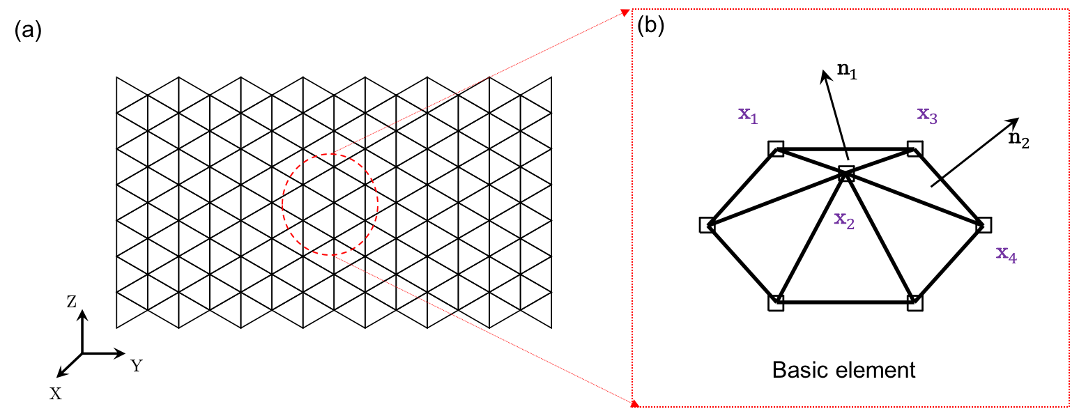
As shown in the figure below, the configuration of a 3D surface is represented by \(N\) nodes, where each node is defined as \(\mathbf{x}_{i} \equiv [x_{i}, y_{i}, z_{i}]^{T} \in \mathcal{R}^{3 \times 1}\). Thus, the total DOF vector is given by
\[\mathbf{q} = [ \mathbf{x}_1; \mathbf{x}_2; \ldots; {\mathbf{x}_{N}} ] \in \mathcal{R}^{3N \times 1}.\]Two types of elements are used to capture the mechanics of a 3D surface: (i) stretching element, and (ii) bending element. The number of stretching elements is denoted as \(N_{s}\), while the number of bending elements is denoted as \(N_{b}\). If only the stretching elements are considered, bending-dominated plate/shell structures will be reduced to stretching-dominated membrane structures.
Stretching element
The stretching element is comprised of two connected nodes, defined as
\[\mathcal{S}: \{\mathbf{x}_{1}, \mathbf{x}_{2} \}.\]The local DOF vector is defined as
\[\mathbf{q}^{s} \equiv [\mathbf{x}_{1}; \mathbf{x}_{2} ] \in \mathcal{R}^{6 \times 1}.\]The edge length is the \(\mathcal{L}_{2}\) norm of the edge vector, defined as
\[l = || \mathbf{x}_{2} -\mathbf{x}_{1} ||.\]The stretching strain is based on the uniaxial elongation of the edge, defined as
\[{\varepsilon} = { l } - \bar{l}.\]Hereafter, we use a bar on top to indicate the evaluation of the undeformed configuration, e.g., \(\bar{l}\) is the edge length before deformation. Using the linear elastic model, the total stretching energy is in a quadratic form of the strain following the linear elastic constitutive law
\[E^s = \frac{\sqrt{3}}{4} Eh ( \varepsilon )^2,\]where \(E\) is the Young’s modulus and \(h\) is the thickness. Note that the Poisson’s ratio is intrinsically determined in this model and equals \(\nu=1/3\) when the mesh is an equilateral triangle. The local stretching force vector, \(\mathbf{F}^{s}_{\mathrm{local}} \in \mathcal{R}^{6 \times 1}\), as well as the local stretching Hessian matrix, \(\mathbb{K}^{s}_{\mathrm{local}} \in \mathcal{R}^{6 \times 6}\), can be derived through a variational approach as
\[\mathbf{F}^{s}_{\mathrm{local}} = -\frac{\partial E^{s}} {\partial \mathbf{q}^{s}}, \; \mathrm{and} \; \mathbb{K}^{s}_{\mathrm{local}} = \frac {\partial^2 E^{s}} {\partial \mathbf{q}^{s} \partial \mathbf{q}^{s}}.\]The detailed formulation can be found in the MATLAB code. Finally, the global stretching force vector, \(\mathbf{F}^{s}\), and the associated Hessian matrix, \(\mathbb{K}^{s}\), can be assembled by iterating over all stretching elements.
Bending element
Before constructing the bending element, we first introduce the triangular element used in 3D surface simulation. Each triangular element has \(3\) vertices as
\[\mathcal{T}: \{ \mathbf{x}_{1}, \mathbf{x}_{2}, \mathbf{x}_{3} \}.\]When two neighboring triangular elements share a common edge (i.e., two common nodes), a bending element is formed to capture the angular deviation between them as
\[\mathcal{B}: \{ \mathcal{T}_{1}, \mathcal{T}_{2} \}, \; \mathrm{with} \; \mathcal{T}_{1} : \{ \mathbf{x}_{1}, \mathbf{x}_{2}, \mathbf{x}_{3} \} \; \mathrm{and} \; \mathcal{T}_{2} : \{ \mathbf{x}_{2}, \mathbf{x}_{3}, \mathbf{x}_{4} \},\]where \(\{ \mathbf{x}_{2} , \mathbf{x}_{3} \}\) are the joint nodes, and \(\{ \mathbf{x}_{1}, \mathbf{x}_{4} \}\) are the two other nodes. Therefore, the local DOF vector is defined as
\[\mathbf{q}^{b} \equiv [\mathbf{x}_{1}; \mathbf{x}_{2};\mathbf{x}_{3};\mathbf{x}_{4} ] \in \mathcal{R}^{12 \times 1}.\]The edge vectors are given by
\[\mathbf{e}_{1} = \mathbf{x}_{2} -\mathbf{x}_{1}, \; \mathbf{e}_{2} = \mathbf{x}_{3} -\mathbf{x}_{1}, \; \mathbf{e}_{3} = \mathbf{x}_{2} -\mathbf{x}_{4}, \; \mathbf{e}_{4} = \mathbf{x}_{3} -\mathbf{x}_{4}.\]Next, the surface normal vectors of two triangular meshes are given by
\[\mathbf{n}_1 = \frac {\mathbf{e}_{1} \times \mathbf{e}_{2}} { || \mathbf{e}_{1} \times \mathbf{e}_{2}||}, \; \mathbf{n}_2 = \frac {\mathbf{e}_{3} \times \mathbf{e}_{4}} {|| \mathbf{e}_{3} \times \mathbf{e}_{4} ||}.\]The bending curvature is associated with the turning angle between the two connecting surfaces, which can be expressed as
\[{\kappa} = || \mathbf{n}_{1} - \mathbf{n}_{2} ||.\]The discrete bending energy is given in a similar approach
\[E^b = \frac{1}{12\sqrt{3}} Eh^3 (\kappa - \bar{\kappa} )^2.\]The local bending force vector, \(\mathbf{F}^{b}_{\mathrm{local}} \in \mathcal{R}^{12 \times 1}\), as well as the local bending Hessian matrix, \(\mathbb{K}^{s}_{\mathrm{local}} \in \mathcal{R}^{12 \times 12}\), can be derived through a variational approach
\[\mathbf{F}^{b}_{\mathrm{local}} = -\frac{\partial E^{b}} {\partial \mathbf{q}^{b}}, \; \mathrm{and} \; \mathbb{K}^{b}_{\mathrm{local}} = \frac {\partial^2 E^{b}} {\partial \mathbf{q}^{b} \partial \mathbf{q}^{b}}.\]The detailed formulation can be found in the MATLAB code. Finally, the global bending force vector, \(\mathbf{F}^{b}\), and the associated Hessian matrix, \(\mathbb{K}^{b}\), can be assembled by iterating over all bending elements.